Decision errors and the value of pre-commitment

Firms employ stage-gates where information is evaluated before deciding to continue resource commitment toward a project. This approach, wherein investments are not fully ex-ante allocated, has the benefit of being more flexible and deferring resource commitments till better information is available. Still, does such flexibility come at a cost? One can come up with some obvious costs, such as the cost of making decisions (and perhaps costs due to associated delays in making decisions). In addition, stage-gate decision making might also suffer from some well-understood biases (such as the escalation of commitment, see for instance ).

But barring biased decisions (or “decision costs” noted above), is there any reason to ever choose to pre-allocate the resources instead of taking a more flexible wait-and-see approach? The model below offers a very distinct reason for why commitment might be of value. Specifically, it demonstrates that when people’s decisions are noisy, it might be better to pre-commit to the resource allocations.

To make the ideas concrete, consider a decision maker who has a single project that she expects to have value of either \(0\) or \(V\) with equal probability. Moreover, suppose the total cost of completing the project is \(c\). We shall consider a 2-stage development process, with both stages costing \(\frac{c}{2}\) and a single stage-gate in between these stages. We shall assume that the true value of the project is revealed at the end of stage \(1\) (so that the decision at stage-gate can be based on this new information revealed from stage 1). Finally, to focus on the interesting cases, we shall assume that \(\frac{V}{2}\ge c\).

First consider the case of optimal decisions:

• If the decision maker has to pre-commit all resources (i.e., the stage-gate does not exist), then the expected value of the project is obviously \(\frac{1}{2}V-c\) if she pursues it, and \(0\) otherwise. Hence, the optimal payoffs with pre-commitment is \(\left(\frac{1}{2}V-c\right)^{+}=\frac{V}{2}-c\)

• If the decision maker can choose at the stage-gate whether to continue the project or not, then she would obviously choose not to pursue if the true value turned out to be \(0\), and would choose to pursue the project if the true value turned out to be \(V\). That is, the expected value (before starting the project) is given by \(-\frac{c}{2}+\frac{1}{2}\left(0\right)+\frac{1}{2}\left(V-\frac{c}{2}\right)=\frac{1}{2}V-\frac{3}{4}c\)

Obviously, the expected payoffs in the flexible approach (with the stage-gate) is higher than in the commitment approach. And if the decision maker can choose the optimal action at every stage, she should opt for the flexible approach.

Now consider the case where the decision maker has a “trembling hand,” i.e., while she is more likely to make the better decision, she might also make a suboptimal decision at every stage. We shall model such decision errors by assuming that when faced between choices \(i\) (\(i=1,\cdots)\) with utilities \(U_{i}\) respectively, the decision maker chooses option \(i\) with probability

where \(\beta\) (\(>0\)) represents the noisiness of the decision in that when \(\beta\rightarrow0\), the persion always makes the decision that yields the highest utility. As may be noted, the above specification is identical to the classic quantal choice models and can be microfounded by assuming an unbiased noise in the assessment of utilities.

With this model of noisy decisions, the expected payoffs in the pre-commit resources and flexible stage-gate settings are as follows

pre-commit resources: The expected utility from pursuing the project is \(\frac{V}{2}-c\) and expected utility from not pursuing the project is \(0\). Hence, the probability that the decision-maker pursues the project is given by \(\frac{\exp\left(\frac{1}{\beta}\left(\frac{V}{2}-c\right)\right)}{\exp\left(\frac{1}{\beta}\left(\frac{V}{2}-c\right)\right)+1}\). Consequently, the expected payoff is given by

flexible stage-gate approach: At the stage-gate, if the true value was revealed to be \(V\), then the decision-maker pursues the project with probability \(\frac{\exp\left(\frac{1}{\beta}\left(V-\frac{c}{2}\right)\right)}{\exp\left(\frac{1}{\beta}\left(V-\frac{c}{2}\right)\right)+1}\) and receives payoff \(\left(V-\frac{c}{2}\right)\); and with remaining probability does not pursue the project and receives payoffs \(0\). Similarly, if the true value was revealed to be \(0\), then the decision-maker pursues the project with probability \(\frac{\exp\left(\frac{1}{\beta}\left(-\frac{c}{2}\right)\right)}{\exp\left(\frac{1}{\beta}\left(-\frac{c}{2}\right)\right)+1}\) and receives payoff \(\left(-\frac{c}{2}\right)\); and with remaining probability does not pursue the project and receives payoffs \(0\). Thus, the expected payoff upon reaching the stage-gate is given by \(\frac{1}{2}\left(\frac{\exp\left(\frac{1}{\beta}\left(V-\frac{c}{2}\right)\right)}{\exp\left(\frac{1}{\beta}\left(V-\frac{c}{2}\right)\right)+1}\left(V-\frac{c}{2}\right)\right)+\frac{1}{2}\left(\frac{\exp\left(\frac{1}{\beta}\left(-\frac{c}{2}\right)\right)}{\exp\left(\frac{1}{\beta}\left(-\frac{c}{2}\right)\right)+1}\left(-\frac{c}{2}\right)\right)\)

When viewed before the first stage, we can make one of two assumptions about the decision-makers knowledge about their own noisy decisions. Specifically, we can assume that she either knows that her 2nd stage decisions are noisy and account for this to calculate her future utility, or she is unaware that her future decisions are noisy. Below, we adopt the “unaware” about future noisy decisions assumption. Still, it should be noted that this behavioral assumption is not critical for the main insight to hold.

Given our assumption (that decision-maker is unaware of her noisy decisions), when the decision-maker, before stage 1, will predict that her utility by choosing to proceed with the project is \(-\frac{c}{2}+\frac{1}{2}\left(V-\frac{c}{2}\right)+\frac{1}{2}\left(0\right)=\frac{V}{2}-\frac{3c}{4}\). Consequently, the probability that she will decide to proceed with the project in the 1st stage is given by \(\frac{\exp\left(\frac{1}{\beta}\left(\frac{V}{2}-\frac{3c}{4}\right)\right)}{\exp\left(\frac{1}{\beta}\left(\frac{V}{2}-\frac{3c}{4}\right)\right)+1}\). Consequently, the actual expected payoffs is given by

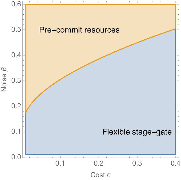
Figure below shows how \(\Pi_{f}\) compares to \(\Pi_{c}\). As may be noted, the decision-maker obtains a higher expected payoff by pre-commiting resources (and giving up her flexibility) when the noise \(\beta\) in her decision is sufficiently large.

Note1: We had assumed that the decision-maker is unaware of the noise in their future decisions. If alternatively, we assume that the decision-maker is aware and accounts for the noise in her decision, then her probability of starting the project (under the flexible stage-gate approach) would become \(\frac{\exp\left(\frac{1}{\beta}u\right)}{\exp\left(\frac{1}{\beta}u\right)+1}\) where \(u=-\frac{c}{2}+\frac{1}{2}\left(\frac{\exp\left(\frac{1}{\beta}\left(V-\frac{c}{2}\right)\right)}{\exp\left(\frac{1}{\beta}\left(V-\frac{c}{2}\right)\right)+1}\left(V-\frac{c}{2}\right)\right)+\frac{1}{2}\left(\frac{\exp\left(\frac{1}{\beta}\left(-\frac{c}{2}\right)\right)}{\exp\left(\frac{1}{\beta}\left(-\frac{c}{2}\right)\right)+1}\left(-\frac{c}{2}\right)\right)\) (instead of \(u=\frac{V}{2}-\frac{3c}{4}\) that we assumed in the unaware case). Thus, while the expression for \(\Pi_{f}\) would be significantly more complicated, the regions corresponding to when flexible approach dominates the pre-commitment approach is nearly identical.

Note2: The story above uses the context of projects and stage-gates. Interestingly, the argument applies for much more general settings of flexibility and commitment. In specific, I discovered this when I was looking at how noisy decisions affect the optimality of sequential vs. parallel testing strategies. In this setting, it turns out that sequential testing, which has the flexibility to stop at any point, is inferior to parallel testing when the noise in decisions in significant. So it appears that “forgo flexibility when decisions are noisy” is much more general phenomenon!