Efforts in Internal Contests

Consider a firm which has two employees. We assume that the employees can either work on routine projects and put in efforts \(E_{i}\) (\(i = 1,2\)), in which case, the firm obtains reward \(E_{1} + E_{2}\) from these routine projects, and the employees obtain wages \(wE_{i}\). Note that for a routine project, the outcome is highly correlated to the efforts, so the above assumption on wages only mean that the firm is paying the employees a piece-rate wage.

The firm also runs a contest with reward \(V\), for which the employees can put in efforts \(e_{i}\). Specifically, when they put in effort \(e_{i}\), the chance that they win the contest is \(\frac{e_{i}e_{- i}}{2} + e_{i}\left( {1 - e_{- i}} \right)\). This reward structure can be easily interpreted in terms of probability of obtaining a certain “solution quality.” For instance, when an employee puts in effort \(e_{i}\), he obtains a solution of quality \(Q\) with probability \(e_{i}\), and with remaining probability \(1 - e_{i}\), he obtains a solution of quality \(0\). And the firm rewards whoever obtains the solution \(Q\), and randomly breaks the tie if both obtain it.

Note that in this conceptualization, the firm’s “revenue” is given by \(E_{1} + E_{2} + \left( {1 - \left( {1 - e_{1}} \right)\left( {1 - e_{2}} \right)} \right)Q\) and cost by \(w\left( {E_{1} + E_{2}} \right) + V\left( {1 - \left( {1 - e_{1}} \right)\left( {1 - e_{2}} \right)} \right)\)

The employees optimization problem is \(\max\limits_{e_{1}E_{1}}wE_{1} + \frac{e_{1}e_{2}}{2} + e_{1}\left( {1 - e_{2}} \right) - \lambda\left( {e_{1} + E_{1}} \right)^{2}\).

NOTE: We have assumed that the cost for the employee is quadratic \(\lambda\left( {e_{1} + E_{1}} \right)^{2}\).

The equilibrium effort levels are given by \(e_{1} = e_{2} = 2\left( {1 - \frac{\lambda}{V}} \right)\) and \(E_{1} = E_{2} = \frac{\lambda}{2} - 2\left( {1 - \frac{\lambda}{V}} \right)\) [NOTE: We need to worry about the boundary conditions, which I am not doing now (since I am too lazy)]

So the firms revenues is given by

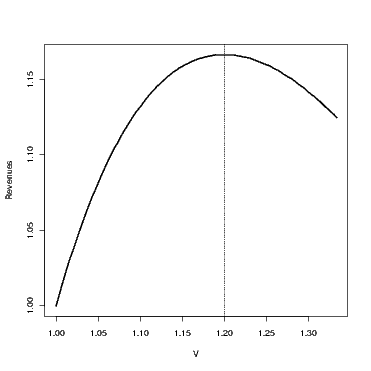
It is interesting to note that the revenues are not increasing in \(V\), and that there is an optimal \(V\) at which the revenues are maximized.

As an example, consider \(\lambda = 1\) and \(Q = 1.5\) Figure below shows the revenue as a function of \(V\). As may be verified, the revenues are maximized when \(V = 1.2\)

This means that even if the firm does not incur the cost of rewarding the employees, (for instance, the reward is perhaps status-related,) holding contests with high rewards is detrimental. We could probably work out how this changes with number of employees, and show that this becomes an even bigger problem with more employees.

Also, it is interesting to note that since the marginal value from routine project is \(w\) and the marginal value from the radical project (if there is no contest) is \(V\), our employees would either work on the routine project, or on the radically new risky one, but not both. But with competition, they would allocate their time on both.

Alternate model:

One concern regarding the above model might be that the contest has only binary outcomes (Q or 0).

Now consider a more general model where performance \(P_{i} = e_{i} + \epsilon_{i}\) where \(\left. \epsilon_{i} \right.\sim N\left( {0,\sigma} \right)\). The remaining part of the model remains as is.

Then, we can show that (if it exists) there is an equilibria in pure strategies where \(e_{1} = 0\) and \(e_{2} = f^{- 1}\left( \frac{\lambda}{V} \right)\) and \(E_{1} = \frac{\lambda}{2}\) and \(E_{2} = \frac{\lambda}{2} - f^{- 1}\left( \frac{\lambda}{V} \right)\). There are other pure strategy equilibria as well. For instance, we can set \(e_{1} = \phi\) and \(e_{2} = f^{- 1}\left( \frac{\lambda}{V} \right) + \phi\), and \(E_{1} = \frac{\lambda}{2} - \phi\) and \(E_{2} = \frac{\lambda}{2} - \phi - f^{- 1}\left( \frac{\lambda}{V} \right)\)). We wont concern ourselves with these equilibria since they all involve the contestants putting in greater effort. So the first equilibria is in fact the pareto optimal equilibria as far as the contestants are concerned.

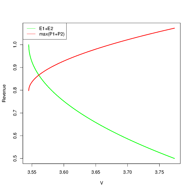
With this structure, we can once again plot out the firm’s payoffs at equilibrium where the revenue from incremental projects is \(E_{1} + E_{2}\), and for the one from radical projects is \(\max\left\{ {P_{1},P_{2}} \right\}\). Figure below plots this for the case of \(\lambda = 1\), \(\sigma = 1\). As may be noticed, the basic structure of the results are fairly robust. As prize money increases, people put less and less effort into routine projects.