Newsvendor Model with Defects

Posted on Wed 07 May 2014 in Core OM and supply chain

How does a retailers order quantity change when his supplier sends products some of which are defective? To answer this question in a concrete context, consider the canonical newsvendor model - demand $D$ is random and has cdf $F\left( \cdot \right)$; cost per unit when the firm places orders is $c$; the price at which the units are sold is $p$ per unit. Assume that there is no salvagage value at the end of the period, and as in the canonical model that the firm has to place the order before the actual demand realization. Then, the (expected) profit maximizing order quantity

$$\begin{array}{llll} Q^{*} & = & {F^{- 1}\left( \frac{p - c}{p} \right)} & \\ \end{array}$$

Now in the canonical newsvendor model make the following modification - assume that when the firm orders $Q$, among the actual $Q$ units that are delivered, a fraction $d$ are defective and cannot be sold. That is, when firm orders $Q$, the number of units of “sellable” stock she has is $\left( {1 - d} \right)Q$. Also, for the sake of focusing on key drivers, assume that the defectives cannot be returned to the supplier and that the firm will end up paying $cQ$ when she orders $Q$. Then, what is the new optimal order quantity?

Naive intuition suggested to me that the firm might need to order more (relative to the case when there are no defects) to make up for the defects. The model below explores if this intuition is true.\

In the model as posed above (with defect rate of $\rho$), the expected profit when the firm orders $Q$ is given by

$$\begin{array}{llll} {\Pi\left( Q \right)} & = & {E\left\lbrack {- cQ + \min\left\{ {D,\left( {1 - \rho} \right)Q} \right\}} \right\rbrack} & \\ \end{array}$$

Hence, the optimal order quantity is

$$\begin{array}{llll} Q^{*} & = & {\arg\max\limits_{Q}\Pi\left( Q \right)} & \\ & = & {\arg\max\limits_{Q}E\left\lbrack {- cQ + \min\left\{ {D,\left( {1 - \rho} \right)Q} \right\}} \right\rbrack} & \\ \end{array}$$

Let $Q^{\prime} = \left( {1 - \rho} \right)Q$ and $c^{\prime} = \frac{c}{1 - \rho}$. Then, the above optimization problem could be rewritten as

\max\limits_{Q^{\prime}}E\left\lbrack {- c^{\prime}Q^{\prime} + \min\left\{ {D,Q^{\prime}} \right\}} \right\rbrack

Since the above is the standard expected profit equation in the canonical newsvendor model, the optimal $Q^{\prime}$ is given by $Q^{\prime} = F^{- 1}\left( \frac{p - c^{\prime}}{p} \right) = F^{- 1}\left( \frac{p - \frac{c}{1 - \rho}}{p} \right)$, and thus the optimal order quality

$$\begin{array}{llll} Q^{*} & = & {\frac{1}{1 - \rho}Q^{\prime}} & \\ Q^{*} & = & {\frac{1}{1 - \rho}F^{- 1}\left( \frac{p - \frac{c}{1 - \rho}}{p} \right)} & \\ \end{array}$$

Interestingly, while the first term $\frac{1}{1 - \rho}$ increases with defects $\rho$, the second term$F^{- 1}\left( \frac{p - \frac{c}{1 - \rho}}{p} \right)$ decreases with defects $\rho$. More specifically, consider the derivative

\frac{dQ^{*}}{d\rho} = \frac{1}{\left( {1 - \rho} \right)^{2}}\left( {F^{- 1}\left( \frac{p - \frac{c}{1 - \rho}}{p} \right) - \frac{c}{p\left( {1 - \rho} \right)}\frac{1}{f\left( {F^{- 1}\left( \frac{p - \frac{c}{1 - \rho}}{p} \right)} \right)}} \right)

At $\rho = 0$, the derivative is

\left. \frac{dQ^{*}}{d\rho} \right|_{\rho = 0} = F^{- 1}\left( \frac{p - c}{p} \right) - \frac{c}{p}\frac{1}{f\left( {F^{- 1}\left( \frac{p - c}{p} \right)} \right)}

For a uniform distribution of demand, say in $\left\lbrack {\mu - \Delta,\mu + \Delta} \right\rbrack$, the above derivative turns out to be $\mu - \Delta\left( {\frac{4c}{p} - 1} \right)$. That is, the optimal order quantity increases if the mean demand is higher, if the variance is lower, and/or if the margin is lower.

Thus, whether quantity increases or decreases also depends on the margins and more broadly even on the distribution of demand. Figure below illustrates this by showing the quantity as a function of defects for the case where the margins are high (cost is low) and where the margins are low. Specifically, assume that $p = 1$, and $c = 0.25$, and let demand be uniformly distributed between $50$ and $350$.

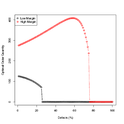
As may be observed, the order quantity increases with defects when the margins are high (red curve), and decreases when the margins are already low (black curve). So I guess the naive intuition turned out to be wrong. A very unscientific poll of operations management students also suggests that people may have the same wrong intuition. I would conjecture that what they are doing is something like this - with deterministic demand, defects imply that we should adjust the order quantity upward. This same intuition is carried over to the case of uncertain demand and people end up thinking that ordering more is in fact the optimal strategy. Perhaps it would be more accurate to say that people sequentially make these choices - for instance, solve it without defects, and then adjust based on what their heuristic tells them to do in the presence of defects. In any case, the model does show that the actual model is much richer than what our naive intuition would suggest.