Noisy decisions and the perils of flexibility

Consider the following: (i) sequential setting: a person who sequentially engages in costly search among alternatives and upon stopping receives the highest value seen so far, and (ii) parallel setting: a person who ex-ante decides the number of alternatives to examine, and then selects the highest value among them.

Obviously, in a “rational” model with payoff maximizers, the sequential setting can never result in lower payoff compared to the parallel setting; since any decision that can be made in the parallel setting can also be made in the sequential setting. Or stated differently in “real options” language, the sequential setting has additional flexibility (including the possibility of stopping earlier or later based on the realized outcomes) compared to the parallel setting. Needless to say, the flexibility should have non-negative value, and thus sequential should always dominate parallel settings. Previous literature, such as Loch et al (2001) suggest that parallel testing cannot dominate unless there is a cost-based advantage (such as parallel testing is less “costly”).

The model below demonstrates a very different “noise-based” channel that can make parallel testing superior to sequential testing (even without any cost advantages).

Suppose that we have 2 alternatives that we can potentially evaluate, and the value of each alternative is ex-ante uncertain and we believe that it is uniformly distributed between \(\left[0,1\right]\). Moreover, suppose that the cost of looking at each alternative is \(c\). We shall assume that people are noisy in their decisions. Specifically, when faced between choices \(i\) (\(i=1,\cdots\)) with utilities \(U_{i}\) respectively, we shall assume that people choose \(i\) with probability

Note that \(\beta\) represents the noisiness of the decision in that when \(\beta=0\), the person will always make the decision that yields higher utility.

Sequential setting: After looking at the 1st alternative, and observing \(x\) (say), we would anticipate that stopping right away gives us \(x\) whereas continuing, we will obtain \(x\times x+\left(1-x\right)\left(\frac{1+x}{2}\right)-c=\frac{1+x^{2}}{2}-c\). As the choices at this stage are between stopping and continuing, based on our assumption of noisy decisions, this person stops with probability

Now consider the decision before starting any evaluation. The person can stop and obtain \(0\), or continue and obtain \(u\left(c\right)=E\left[\max\left\{ x,\left(\frac{1+x^{2}}{2}-c\right)\right\} \right]=\frac{2}{3}-c\left(1-\frac{2\sqrt{2c}}{3}\right)\). Note that the implicit assumption is that the person does not anticipate their noisy decisions in the future. Consequently, their expected payoff will continue is given by \(\Pi_{s}\left(c,\beta\right)=\frac{\exp\left(\frac{u\left(c\right)}{\beta}\right)}{\exp\left(0\right)+\exp\left(\frac{u\left(c\right)}{\beta}\right)}\left(u\left(c\right)-c\right)\)

Parallel testing. The person has the choice between testing none, testing 1 and testing 2. The utility corresponding to these choices are \(0\), \(\frac{1}{2}-c\), and \(\frac{2}{3}-2c\) respectively. Hence, the expected payoff is given by \(\Pi_{p}\left(c,\beta\right)=\frac{\exp\left(\frac{\frac{1}{2}-c}{\beta}\right)}{\exp\left(0\right)+\exp\left(\frac{\frac{1}{2}-c}{\beta}\right)+\exp\left(\frac{\frac{2}{3}-2c}{\beta}\right)}\left(\frac{1}{2}-c\right)+\frac{\exp\left(\frac{\frac{2}{3}-2c}{\beta}\right)}{\exp\left(0\right)+\exp\left(\frac{\frac{1}{2}-c}{\beta}\right)+\exp\left(\frac{\frac{2}{3}-2c}{\beta}\right)}\left(\frac{2}{3}-2c\right)\)

Figure below shows the contingencies when \(\Pi_{s}>\Pi_{p}\). As may be noted, with noisy decisions, parallel can dominate sequential (more flexible) decisions when the cost is low or noise is sufficiently high.

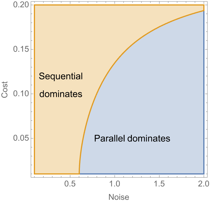
Note: We assumed that the person is not aware of their noisy future decisions. That is, when they make their choice in period 1, they don’t anticipate and factor in their noisy decisions in 2nd period. If however the person factors this in, then in the sequential case we would need to substitute \(u\left(c,\beta\right)\) for \(u\left(c\right)\) where \(u\left(c,\beta\right)=E\left[p\left(x,\beta\right)x+\left(1-p\left(x,\beta\right)\right)\left(\frac{1+x^{2}}{2}-c\right)\right]\). Consequently, their expected payoff is given by \(\Pi_{s1}\left(c,\beta\right)=\frac{\exp\left(\frac{u\left(c,\beta\right)}{\beta}\right)}{\exp\left(0\right)+\exp\left(\frac{u\left(c,\beta\right)}{\beta}\right)}\left(u\left(c,\beta\right)-c\right)\). Even in this case, the broad qualitative result - parallel can dominate sequential when noise is high and cost is low - still continues to hold.