Noisy evaluations and the choice between parallel and sequential testing

Testing many alternatives, with the goal of identifying a single best alternative, can proceed in one of two ways: (i) parallel - where the agent decides on the number of alternatives to examine, and after examining them selects the one that yielded the highest value, or (ii) sequential - where the agent, at each stage, chooses whether to examine one more alternative and upon stopping receives the highest value seen so far.

If the agent can first select between the two modes - parallel and sequential - then, which one would be more profitable?

As the sequential mode has greater flexibility compared to the parallel mode (since one can choose to stop earlier in sequential mode), obviously, if there is no extra benefits associated with parallel tests, then sequential evaluations should always yield higher profits compared to parallel evaluations. Loch et al (2001) offers a model which demonstrated the somewhat obvious insight - parallel testing dominates only when the cost of sequential tests are much larger than the cost of parallel tests, i.e., when delays (because of sequential tests) are costly, one should choose parallel tests.

Beyond the issue of “delay costs,” is there any other contingency that leads to one or the other mode of testing becoming more suitable. Specifically, in a prior paper, I and one of my coauthors had looked at the issue of evaluation noise and how it can affect sequential testing. This blog post is an attempt to analyze how evaluation noise affects the tradeoffs between parallel and sequential testing modes.

Consider a firm that has \(N\) potential prototypes. The firm believes, ex-ante before any evaluations, that every prototype \(i\) (\(i=1,\cdots,N\)) has “true” value \(\mathbf{p}_{i}\) which is distributed normally with mean \(\mu\) and standard deviation \(\sigma\). Upon evaluating a given prototype \(i\) at cost \(c\), the firm obtains a measurement \(\mathbf{m}_{i}=\mathbf{p}_{i}+\mathbf{\epsilon}_{i}\) where \(\epsilon_{i}\) is normally distributed with mean \(0\) and standard deviation \(\frac{1}{\tau}\). Thus, in the above formulation, the fidelity of measurement is captured through \(\tau\) where a high (lower) value represents more (less) precise measurements.

Let \(C=c+c^{\prime}\) be the effective cost incurred during sequential testing upon evaluating each alternative. In this conceptualization, \(c\) represents the actual evaluation cot and \(c^{\prime}\) represents the “cost” of waiting one additional period. Similarly, in the case of parallel tests, the total cost upon testing \(n\) alternatives is given by \(nc+c^{\prime}\) (since all these parallel tests are conducted simultaneously in the first period itself).

While the analysis for figuring out the optimal sequential policy and the optimal parallel tests are somewhat messy, the final solution turns out to be surprisingly simple (see Erat, 2024). Define \(\theta=\sqrt{1+\frac{1}{\sigma^{2}\tau^{2}}}\); then

• The optimal expected value in sequential is given by \(\mu+\frac{\sigma}{\theta}R\left(\left(c+c^{\prime}\right)\frac{\theta}{\sigma}\right)\) where \(R\left(y\right)\) is defined as the solution of \(x=E\left[\max\left\{ x,\mathbf{Z}\right\} \right]-y\) where \(\mathbf{Z}\) is a standard normal distribution.

• The optimal expected value in parallel testing is given by \(\mu-c^{\prime}+\arg\max_{n}\left\{ g\left(n\right)\frac{\sigma}{\theta}-cn\right\}\) where \(g\left(n\right)=E\left[\max_{i=1,\cdots,n}\mathbf{Z_{i}}\right]\).

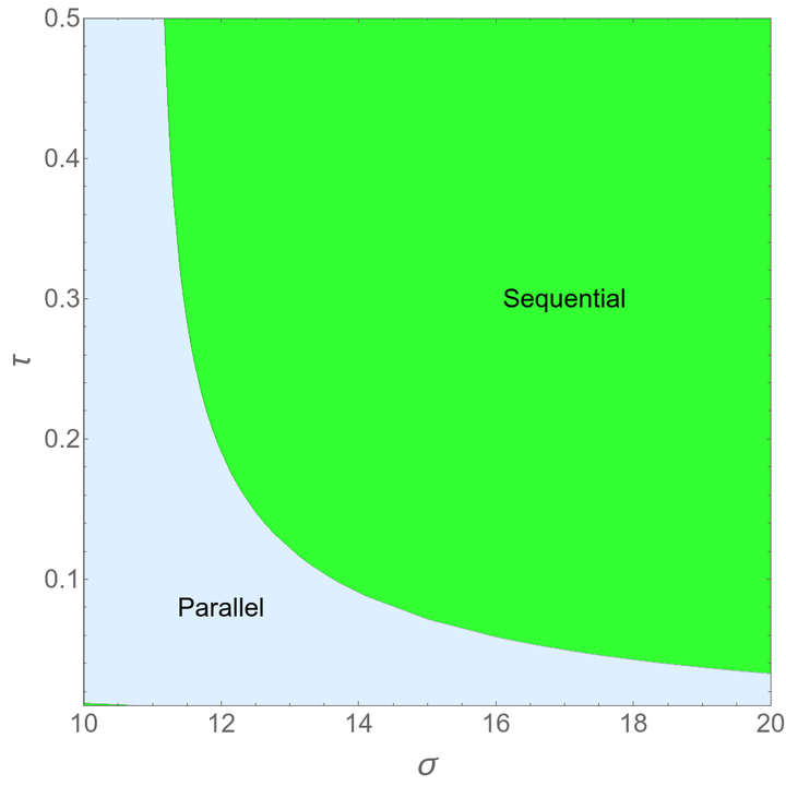
Figure below shows which of these - parallel or sequential - would result in higher profits. So to answer our question,

Parallel tests dominates sequential tests when the fidelity of evaluations is sufficiently low and when the uncertainty in evaluations is small.